SBI for SGWB
Simulation based infernce for Stochastic GW background Analysis (Alvey+, 2023)
NZ Gravity Journal Club
Oct 26th, 2023
Summary
- LISA “Global fit” + GW background
- Alvey+’s LISA SGWB model
- Sim based inference + TMNRE
- Results, Discussion + future work
LISA Data analysis
The data
The “Global fit”
Analyze all the data, simultaneously, block-by-block
$<10^5$ parameters in the full problem
SGWB estimation methods
| Noise model | Signal model | Noise + Signal |
|---|---|---|
| Karnesis+ ‘19 | Baghi+ ‘23 | Boileau+ ‘20 |
| Caprini+ ‘19 | Muratore+ ‘23 | Olaf+ ‘23 |
| Pieroni+ ‘20 | Aimen+ (WIP) |
High precision reconstruction required to extract an SGWB signal
Alvey+’s SBI approach motivations
Note:
- Current SGWB approaches use stochastic sampling methods (MCMC, Nested sampling)
- These are not robust to foreground transient signals (e.g. massive BH mergers)
- add more comlexities
- ‘Marginal inference’ property
- Likelihood ‘free’ inference
- More robust to foreground transient signals (e.g. massive BH mergers)
SBI
Traditional problem
$$ p(\theta|d) = \frac{\mathcal{L}(d|\theta)\pi(\theta)}{\color{red}{Z(d)}}= \frac{\mathcal{L}(d|\theta)\pi(\theta)}{\color{red}{\int_{\theta}\mathcal{L}(d|\theta)\pi(\theta) d\theta}} $$- Monte Carlo: e.g. Rejection sampling
- Markov-chain MC: e.g. Metropolis-Hastings, NUTS
- Variational Inference: surrogate $p(\theta|d)$
What if we dont have $\mathcal{L}(d|\theta)$ ?
Simulation based inference:
New term for:
- Approximate Bayes Computation,
- Likelihood free inference,
- Indirect inference,
- Synthetic likelihood
Algorithm
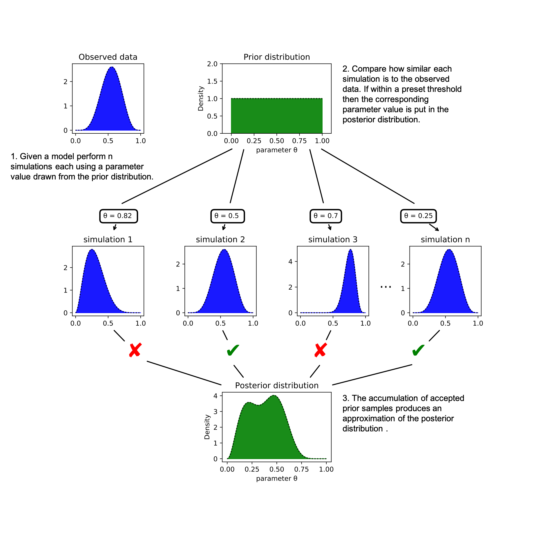
Compare the ‘simulated’ data to the ’true’ data
Note:
- Marginal inference – SBI its possible to directly target specific parameters for inference, ignore other parameters while still dealing correctly with the ones we dont care about
- Amortized – SBI once trained – we can get answers of the posteriors very quickly
Different SBI methods:
- Classical: Rejection ABC (‘97), MCMC-ABC (‘03)
- Neural density:
- Neural posterior estimator
- Neural likelihood estimator
- Neural ratio estimator (Lnl/evid)
- Types of NN:
- Mixture density networks
- Normalising flows
Goals for NN + SBI:
- Speed: Training faster than MCMC
- Scalability: Doesn’t fall apart with high D
- Pre-existing research: Leverage modern ML tools (flows, NNs …)
MCMC, VI, SBI
| MCMC | VI | SBI | |
|---|---|---|---|
| Explicit Likelihood | ✅ | ✅ | ❌ |
| Requires gradients | ✅ | (✅) | ❌ |
| Targeted inference | ✅ | ✅ | ❌ |
| Amortized | ❌ | (✅) | ✅ |
| Specialised architechture | ❌ | ✅ | ✅ |
| Requires data summaries | ❌ | ❌ | ✅ |
| Marginal inference | ❌ | ❌ | ✅ |
Note: Amortized posterior is one that is not focused on any particular observation
END OF SECTION
SBI Math
Skipping this, can come back if folks interested
Note: Library: swyft Simulation efficient marginal posterior estimation
Target: X
- say there are lots of parameters $\theta$
- Only parameter values that plausiablly generate X will contribut to marginaliation
- NESTED RATIO ESTIMATION finds this region by iteratively cnstraining the initial prior based on 1D marginal posteriors from previous iterations
- this method approximates the likelihood-to-evidence ratio by zeroing in on the high-likelihood regions
- method inspired by nested sampling
- After a few iteraintins – some 1D marginals will be mre constrained than others
https://pbs.twimg.com/media/E65qN0dWEAAxXCW?format=png&name=900x900
$D_{KL}$ “Loss” function for training
$$D_{\rm KL}(\tilde{p}, p) = \int \tilde{p}(x) \log \frac{\tilde{p}(x)}{p(x)}\ dx$$$D_{KL}$ is not symmetric
- $D_{\rm KL}(\tilde{p}, p)$: Variational inference (LnL based)
- $D_{\rm KL}(p, \tilde{p})$: NPE (Simulation based)
PROBLEM: how do we avoid evaluating the $p(\theta|d)$?
KL-Divergence and VI
$$D_{\rm KL} [\tilde{p}, p] (\theta) \sim \mathbb{E}_{\theta\sim\tilde{p}(\theta|d)} \log \left[ \frac{\tilde{p}(\theta|d)}{\mathcal{L}(d|\theta)\pi(\theta)} \right] + C$$- PROBLEM: $p(\theta|d)$ is $$$
- SOLUTION:
- $p(\theta|d) \sim \mathcal{L}(d|\theta)\pi(\theta)$
- $0\leq D_{\rm KL} [\tilde{p}, p]\leq Z(d)$
- Train $\tilde{p}(\theta|d)$
KL-Divergence and SBI
$$D_{\rm KL}[p, \tilde{p}] (\theta, d) \sim -\mathbb{E}_{(\theta,d)\sim p(\theta,d)} \log \tilde{p}(\theta| d) + C $$- PROBLEM: $p(\theta|d)$ is $$$
- SOLUTION:
- sample from $p_{\rm joint}(\theta, d) = \mathcal{L}(d|\theta)\pi(\theta)$
- Train $\tilde{p}(\theta|d)$
Marginal SBI vs VI
Variatinal inference
- variational posterior $\tilde{p}(\vec{\theta}|d)$ must conver all params likelihoodd model condditioned on
SBI Marginal inference
- Can replace $\tilde{p}(\vec{\theta}|d)$ for $\tilde{p}(\theta_1|d)$ without need of doing integrals
END OF SECTION
“Marginal” inference
$${\color{red}p(\theta_{\rm Waldo}| \rm{image})} =$$$$\int {\color{blue}p(\theta_{A}, \theta_{B} ... \theta_{\rm Waldo}| \rm{image})}\ d\theta_A\ d\theta_B\ d\theta_{\rm Waldo} $$- VI: have to learn whole $\color{blue}p(\vec{\theta}|d)$
- SBI: can focus on specific params $\color{red}p(\theta_{\rm Waldo}|d)$
Truncated Marginal Neural Ratio Estimation (TMNRE)
Active learning loop

Network architecture

Truncation example

Alvey+ Signal and noise model
Noise model (only amplitudes parameterised – shape fixed):
- $\small S^{\rm N}(A, P, f) \sim A^2 s^{TM}(f) + P^2 s^{OMS}(f)$
Two signal models (one chosen):
- $\tiny {\rm Power Law}: \Omega(\alpha, \gamma, f) \sim 10^\alpha\ f^\gamma$
- $\tiny {\rm N-Power Laws}:\Omega(\vec{\alpha}, \vec{\gamma}, \vec{f}_{\rm range}, f) \sim \sum^N 10^\alpha_i\ f^\gamma_i\ \Theta[f_i^{\rm min}, f_i^{\rm max}]$
BASE Model consists of
- data(t) = noise(t) + $\sum^{\rm signals}$ s_i(t)
- Single TDI channel
- 12 days of data (split into 100 segments, 1 segment ~ 2.9 hours)
- $\Delta f\sim0.1\ {\rm mHz}$
Note: this is ~1% of the full LISA mission duration
Model with transients:
- Same as BASE mode
- In each segement Inject 1 massive BH merger (priors below) if U[0,1] < p
    Mc = U(8e5, 9e5)
    eta = U(0.16, 0.25)
    chi1 = U(-1.0, 1.0)
    chi2 = U(-1.0, 1.0)
    dist_mpc = U(5e4, 1e5)
    tc = 0.0
    phic = 0.0
MLA training:
“Several numerical settings should be chosen for the general structure of the algorithm as well as the network architechture”
- 500K simulations (9:1 train:val split)
- 50 epochs (512 batch size)
- save model weights with the lowest validation loss
Results + Discussion
MCMC vs SBI fit

Some thoughts
- The good:
- ‘Implicit marginalisation’ may enable focused study (without global fit)!
- Fewer evaluations of the model needed!
- The $\tiny{\rm bad}$ not so good:
- Doest use LnL even when known (no gradients)
- Requires robust models for noise (slow!)
- Need to model all signals in data generation?
- MLA architecture…
- The ugly:
- unfair MCMC comparison for data with transients
Future work
- More complex noise model
- Longer data duration
- Additional data channels
- other “SBI” blocks for the global fit
Other related papers
- Fast and credible likelihood-free cosmology with TMNRE
- Improved reconstruction of a stochastic gravitational wave background with LISA
- Truncated Marginal Neural Ratio Estimation
- Scalable inference with Autoregressive Neural Ratio Estimation
- Fast Likelihood-free Reconstruction of Gravitational Wave Backgrounds
- More plots