Matched Filtering

Last updated on Apr 27, 2023

Table of Contents

A Conceptual Discussion

Matched filtering in human brains

Human brains do a form of matched filtering when brains classify certain sounds as ‘words’. Eardrums are vibrated by sound waves and brains compare these sound waves to other template sound waves that are known. In the case of words, brains compare the sound waves with a bank of sound waves from learned words. This process is similar to how LIGO data analysts use matched filtering to find gravitational waves in LIGO data.

Matched filtering in LIGO data

Compact binary coalesence (CBC) searches like PyCBC use matched filtering to find gravitational wave signals in LIGO strain data. This method compares a gravitational wave template (numerical values representing one perticular gravitational wave) to strain data. Before the strain data is compared to the gravitational wave template, the data is weighed based on the detector’s sensitivity (lower the weight of the data that comes from a region where the detector is not sensitive). The output of matched-filtering is a signal-to-noise ratio (SNR) that can be used to determine if the data contains something interesting (a potential gravitational wave candidate) or just noise.

There are many possible gravitational wave templates (gravitational waves from CBCs can have 15 parameters that can describe them hence there are $O(n^{15})$ possible templates). To compute a matched-filter SNR for each of these templates with the LIGO data is computationally expensive. Hence, instead of match-filtering with all templates, only a subset of templates to be used in matched-filtering is selected and stored in a template bank. The bank is created to cover as much of the parameter space as possible by storing only the unique looking templates.

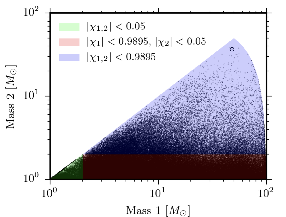
An example template bank used by LIGO searches.

The maths

Optimal detection statistic

The first question LIGO data analysts ask when they receive LIGO strain data $s(t)$ is:

Does the $s(t)$ consist only of noise $n(t)$ or does $s(t)$ contain a gravitational wave signal $h(t)$ hidden in the noise?

The two situations are two different hypotheses about the strain data:

Null Hypothesis, $\mathcal{H}_{n}: n(t) = s(t)$, and
GW Hypothesis, $\mathcal{H}_{GW}: n(t) = s(t) - h(t)$.

Bayes theorem can answer which of the two hypotheses are favoured by the data with an odds ratio: \begin{equation} \label{eq:odds} \begin{split} \mathcal{O}(\mathcal{H}{GW}| s) & = \frac{P(\mathcal{H}{GW}|s)}{ P(\mathcal{H}_{n} | s)} . \end{split} \end{equation}

This odds ratio is the optimal detection statistic that expresses the value of the probability that the data contains the anticipated signal be calculated when

the statistical properties of the noise process are known
the exact form of the signal is known

The following subsections describe in detail the statistical properties of the noise and signal that permit LIGO data analysts to calculate $\mathcal{O}(\mathcal{H}| s)$.

Gaussian noise

To simplify the ability to make a detection, noise $n(t)$ is assumed to be [stationary Gaussian white noise]. For Gaussian white noise time series data that is sampled at regular intervals of $\Delta t$, the probability of collecting a set of $N$ datapoints $\vec{n}$, where $$\vec{n} = \{n_0(t=0), n_1(t=\Delta t), n_2(t=2 \Delta t), …, n_{N-1}(t= (N-1) \Delta t) \}$$ from $0\leq t\leq T$, can be written as: \begin{equation} \label{eq:gaussian} \begin{split} p_n(\vec{n}) &= \prod^{N-1}0 \frac{1}{\sigma\sqrt{2\pi}}\ \text{exp}\left( \frac{-1}{2\sigma^2} n_i^2 \right) \\ &= \frac{1}{(\sigma\sqrt{2\pi})^N}\ \text{exp}\left( \frac{-1}{2\sigma^2} \sum^{N-1}{i=0} n_i^2 \right) \end{split} \end{equation} the following subsections delve into the maths required to simplify this.

Summing samples

For $\lim {\Delta t \to 0}$, $\sum^{N}_{i=1} n_i^2$ turns into an integral:

\begin{equation} \label{eq:gauss_limit} \begin{split} \lim_{\Delta t \to 0} \sum^{N}{i=1} n_i^2 \Delta t &= \int^T_0 n^2(t) dt \\ &= \text{(Parseval’s Theorem and assume $0 \to T$ very large?)} \\ &\approx \int^{-\infty}{+\infty} |\widetilde{n}(f)|^2 df \end{split} \end{equation}

Autocorrelation function for Gaussian Noise

Additionally, as $\lim {\Delta t \to 0}$, we can also get an expression for the autocorrelation function.

Autocorrelation Function:

The autocorrelation function is a tools used to find patterns in time-series data. There are two types:

Ensemble autocorrelation: quantifies correclation between points after repeated trials
Temporal autocorrelation: quantifies correlation between points separated by various time lags in the same time-series

As points become more separated, typically the temporal autocorrelation function should go to 0 (since it is difficult to to forecast further into the future from a given set of data).

For a continuous-time signal $y(t)$ and a lag of $\tau$, the temporal autocorreclation $R^T_{yy}(\tau)$ is given by: $$ R^T_{yy}(\tau) = \int^{+\infty}{-\infty} y(t) y^*(t-\tau)\ ,$$ and the ensemble autocorrelation $R^E{yy}(\tau)$ is given by: $$ R^E_{yy}(\tau) = \langle y(t)|y(t-\tau)\rangle. $$

If the signal is erodic (ie the signal’s statistical properties can be deduced from a long set of random samples), then $$ R^T_{yy}(\tau) =\lim_{T\to \infty} \frac{1}{T} \int^{T}{0} y(t) y^*(t-\tau)dt = R^E{yy}(\tau) .$$

Finally, note that the units ot $R$ are that of power! Hence, this can be used in the calculation of a power spectral density.

At $\lim {\Delta t \to 0}$, the autocorrelation function for $n(t)$ becomes \begin{equation} \label{eq:gauss_autocorrelation_temporal} \begin{split} R^T_{nn}(\tau=\Delta t) &= \lim_{T\to \infty} \frac{1}{T} \int^{T}{0} n(t) n^*(t-\Delta t)dt \\ &= \lim{T\to \infty} \frac{1}{T} \int^{T}_{0} |n(t)|^2 dt \\ &= A\delta(\tau) \end{split} \end{equation}

To determine $A$, we need to consider $R^E_{nn}$. Note for a random process $x(\theta)$, $$ \langle x(\theta)|x(\theta) \rangle = \mu$$ $$ \langle (x(\theta)-\mu)^2| (x(\theta)-\mu)^2 \rangle = \sigma^2$$ Hence, for Gaussian white noise where $\mu=0$,

\begin{equation} \label{eq:gauss_autocorrelation_ensemble} \begin{split} \sigma^2 &= \langle (n(t)-\mu)^2| (n(t)-\mu)^2 \rangle\rangle \\ &= \langle n^2(t)| n^2(t) \rangle\rangle \\ &= R^E_{nn}(\tau) \\ &= A \end{split} \end{equation}

Thus, $$R_{nn}(\tau)=\sigma^2\delta(\tau) $$

Power spectral density from autocorrelation

The one-sided power spectral density $\text{PSD}(f)$ (of a signal $n(t)$) is defined as twice the Fourier transform of the noise autocorrelation function: \begin{equation} \label{eq:psd_calc} \begin{split} \text{PSD}(f) &= 2 \mathcal{F}(R_{nn}(t))) \\ &= 2 \int_{-\infty}^{+\infty}R_{nn}(\tau) e^{-if\tau}d\tau \end{split} \end{equation}

Derivation of the above PSD equation (taken from Mike Lau’s master’s thesis) \begin{equation} \label{eq:psd_derivation} \begin{split} \mathcal{F}(R_{nn}(t))) &= \langle \tilde{n}^*(f) \tilde{n}(f’)\rangle\\ &= \iint^{\infty}{-\infty} \langle {n}(t) {n}(t’)\rangle e^{-2\pi i (ft-f’t’)} dt dt’\\ &{t’\to t+t’}\\ &=\iint^{\infty}{-\infty} \langle {n}(t) {n}(t+t’)\rangle e^{-2\pi i(f-f’)t} e^{-2\pi if’t’} dt dt’\\ &=\int^{\infty}_{-\infty} \langle {n}(t) {n}(t+t’)\rangle e^{-2\pi if’t’} dt’ \delta(f-f’) \\ &= \frac{1}{2}\text{PSD}(f)\delta(f-f’) \\
\end{split} \end{equation}

In the case where $\lim {\Delta t \to 0}$, $$R_{nn}(\tau)=\sigma^2\delta(\tau) = R_{nn}(f), $$ hence, $$\text{PSD}(f) = \lim_{\Delta t \to 0} 2\sigma^2 \Delta t$$

Gaussian noise at $\lim {\Delta t \to 0}$

Finally, putting the above together, the probability of collecting a set of $N$ datapoints $\vec{n}$ from Guassian white noise is simplified to: \begin{equation} \label{eq:gaussian_prob} \begin{split} p_n(\vec{n}) &= \lim_{\Delta t \to 0}\frac{1}{(\sigma\sqrt{2\pi})^N}\ \text{exp}\left( \frac{-1}{2\sigma^2} \sum^{N-1}{i=0} n_i^2\right) \\ &\propto \lim{\Delta t \to 0} \text{exp}\left( \frac{-1}{2\sigma^2\Delta t} \sum^{N-1}{i=0} n_i^2 \Delta t\right) \\ &\propto \text{exp}\left( \frac{-1}{\text{PSD}(f)} \int^{T}{0} n(t)^2 dt\right) \\ &\propto \text{exp}\left( - \int^{\infty}{-\infty} \frac{|n(f)|^2}{\text{PSD}(f)} df\right) \\ &\propto \text{exp}\left(-\frac{1}{2} 4 \int^{\infty}{0} \frac{|n(f)|^2}{\text{PSD}(f)} df\right) \\ \therefore p_n(\vec{n}) &\propto \text{e}^{-(n,n)/2} \end{split} \end{equation}

**Noise Weighted Inner product of two time-series ** The noise weighted inner product $(a,b)$ of two time-series $a(t)$ and $b(t)$ is defined as \begin{equation} \label{eq:inner_producs} \begin{split} (a,b) &= 4 \text{Re} \int_0^{\infty} \frac{\tilde{a}(f) \tilde{b}^(f)}{\text{PSD}(f)}df\\ &= 2 \int_{-\infty}}^{\infty} \frac{\tilde{a}(f) \tilde{b}^(f)}{\text{PSD}(|f|)}df\\ &= \int_{-\infty}}^{\infty} \frac{\tilde{a}(f) \tilde{b}^(f) + \tilde{a}^(f) \tilde{b}(f)}{\text{PSD}(|f|)}df, \end{split} \end{equation}

where

$\text{PSD}(f) is the one-sided power spectral density of noise, and
$\tilde{y}(-f) = \tilde{y}^*(f)$ .

Matched-Filter

The above section provides a mathematical perscription to calculate the probability desnsity that a collection of time-series data comes from stationary Gaussian white noise. Using this, the probability density of getting some data given $\matchcal{H}{n}$ and the probability density of getting some data given $\matchcal{H}{GW}$ can be calculated:

$p(s|\mathcal{H}_{n}:n=s) \propto \text{e}^{-(s,s)/2}$
$p(s|\mathcal{H}_{GW}:s=s-h) \propto \text{e}^{-(s-h,s-h)/2}$

Finally, going off of the odd’s ratio, we can calculate a likelihood ratio:

\begin{equation} \label{eq:likelihood_ratio} \begin{split} \Lambda(\mathcal{H}{GW}| s) &= \frac{p(s|\mathcal{H}{GW}|s)}{ p(s|\mathcal{H}_{n})} \\ &= \frac{\text{e}^{-(s-h,s-h)/2}}{\text{e}^{-(s,s)/2} \\ &= \text{e}^{(s,h)}\text{e}^{-(h,h)/2} \end{split} \end{equation}

Note that:

$\Lambda(\mathcal{H}_{GW}| s)$ depends on the data $s(t)$ only through $(s, h)$
$\Lambda(\mathcal{H}_{GW}| s)$ is a monotonically increasing function of this $(s, h)$.

$\therefore (s,h)$ is the optimal detection statistic: any choice of threshold on the required odds ratio for accepting the alternative hypothesis can be translated to a threshold on the value of $(s, h)$. This inner produc is the matched filter since it is a noise-weighted correlation of the anticipated signal with the data.

The code

As discussed above, one method of searching for a specific signal in a noisy data is via a matched filter. The code for this is illustrated in this section.

Defining signals and noise

Here is the python code to generate Gaussain pulses, square pulses and noise.

def get_gaussian_pulse_signal(time: np.ndarray) -> np.ndarray:
  sig = scipy.signal.gausspulse(t=time, fc=5)
  sig[np.abs(sig) < 1e-2] = 0
  return sig


def get_square_pulse_signal(time: np.ndarray) -> np.ndarray:
  idx_to_one = np.abs(time) <= 0.5
  sig = np.array([1 if one else 0 for one in idx_to_one])
  return sig


def get_noise(time: np.ndarray, noise_factor: Optional[float] = 2) -> np.ndarray:
  noise = np.random.randn(1, len(time)) * noise_factor
  return noise[0]

The data generated from Gaussian noise and a Gaussian Pulse signal is shown in the following image.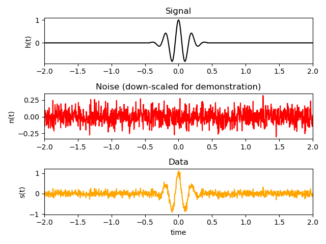

A demonstrative image showing what happens to a Gaussian Pulse signal when some noise is added to it.

Defining the matched-filtering code

Here is a rudimentary implementation of a matched-filter method, where the data is multiplied with the template, and the convolution is summed.

def perform_matched_filter(
  time: np.ndarray,
  data: np.ndarray,
  template_func: Callable
) -> Dict:
  match_filter_values = []
  template = move_template_to_lowest_time(t=template_func(time))

  for i in range(0, len(data), 10):
    current_template = np.roll(template, shift=i)
    matched_filter = sum(data * current_template)
    match_filter_values.append(dict(
      matched_filter=matched_filter,
      time=time[i],
      template=current_template
    ))
  return match_filter_values